Your First Terrain

This is a hands-on walkthrough: open Hesiod, wire up a small graph, and get a real terrain out the other end — a raw heightmap for your engine and a coloured map to look at. It is the do this first page. If you want the why behind the ideas below, read Core Concepts first; this page is the how.

Every step below is a real action in the app. The node names, ports, and parameters are exactly what you will see on screen.

What you'll build

One short graph. The shape looks linear at first, but it forks at the end: the eroded heightmap feeds two outputs — a raw export and a coloured one.

graph LR
  A["NoiseFbm<br/>(base relief)"] -->|heightmap| B["HydraulicParticle<br/>(erosion)"]
  B -->|heightmap| C["ExportHeightmap<br/>(raw)"]
  B -->|heightmap| D["ColorizeGradient"]
  D -->|texture| E["ExportTexture<br/>(colour)"]

The fork is the one thing newcomers trip over, so it is worth saying plainly: the raw heightmap export branches off before the colouriser, because exporting a heightmap and colouring a heightmap are two different things done to the same data. More on that at Step 4.

Open Hesiod

When Hesiod opens you are looking at three things:

• the node graph in the centre, where you build the graph;
• the 3D viewport, where the terrain is rendered;
• the resolution selector, which controls how finely the terrain is computed.

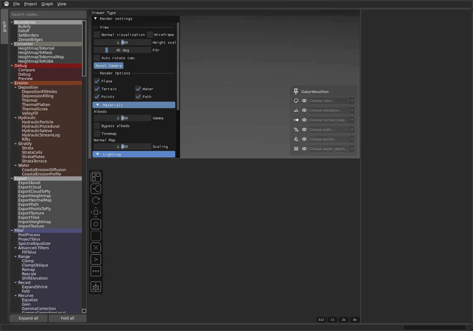
To add a node, open the node library and pick one, or right-click in the graph. Nodes are grouped by category — the categories in parentheses below tell you where to find each one.

Step 1 — A base heightmap (NoiseFbm)

Add a NoiseFbm node (category Primitive/Coherent). This is your starting relief: fractal noise that already looks vaguely landscape-like.

The three knobs worth playing with first:

• seed — change it to get a completely different landscape.
• kw — the wavenumber, i.e. the base feature size. Lower is broader hills; higher is busier terrain.
• octaves — how many layers of detail are stacked on top. More octaves = more fine detail.

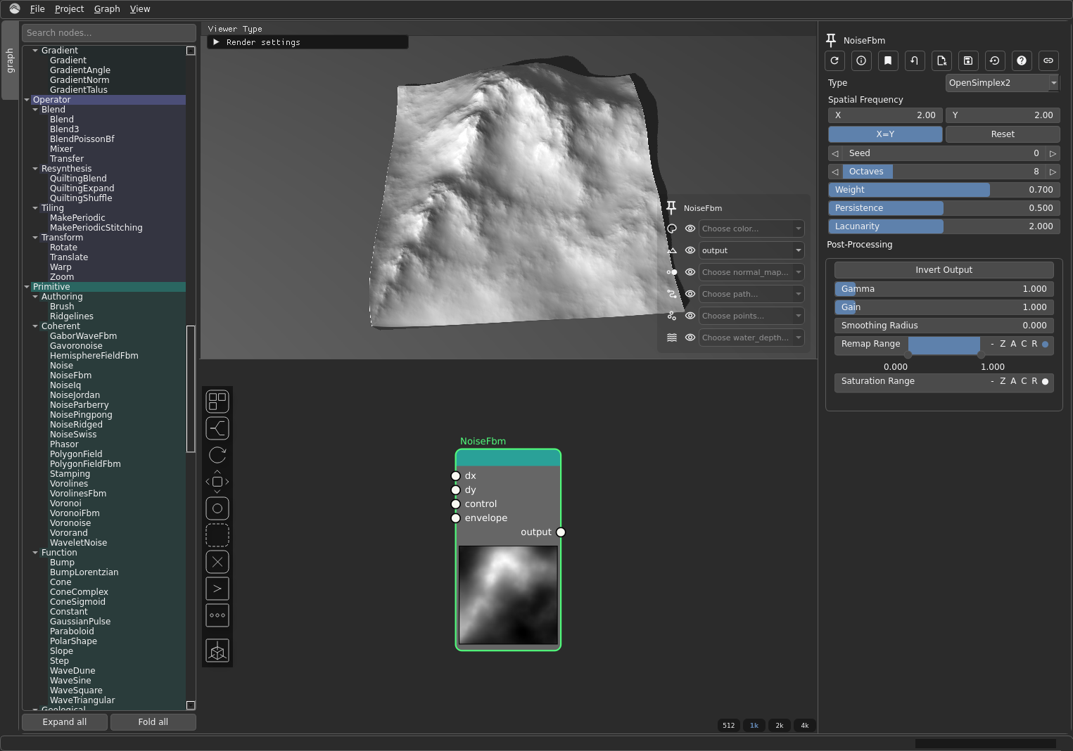
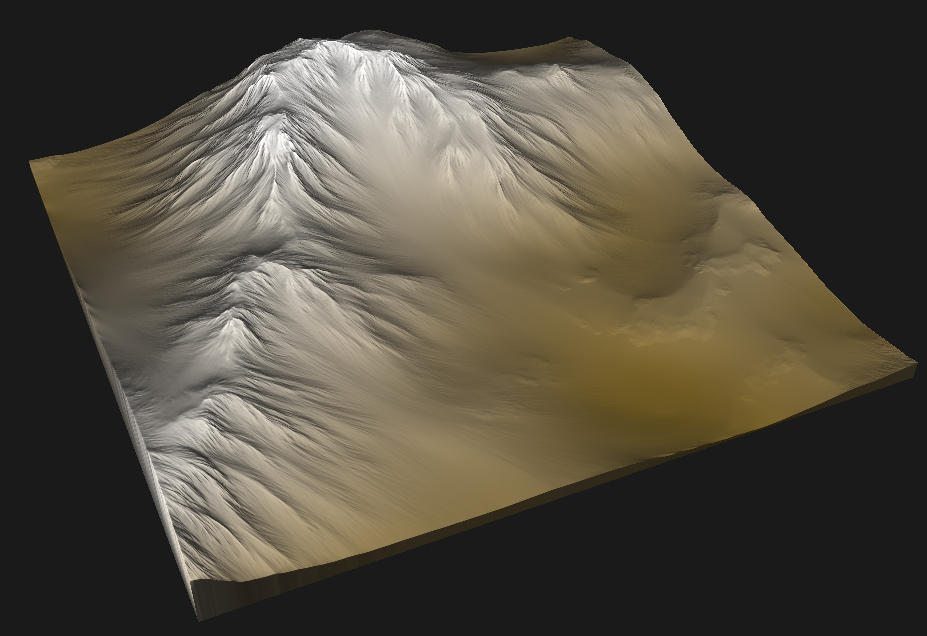
Why: fractal noise gives natural-looking base relief to build on. On its own it is not yet terrain — that comes next.

Reading the previews

Each node shows a small preview thumbnail in its body — a live grayscale (or colour) picture of what that node currently produces. It refreshes as you change settings, so you can dial in a parameter and watch the result. If a preview ever looks stale, the node's settings toolbar has a Force Update button that recomputes it. See the node settings toolbar for the full set of buttons.

Step 2 — Erode it (HydraulicParticle)

Add a HydraulicParticle node (category Erosion/Hydraulic) and wire NoiseFbm's output into the erosion node's input. Erosion is what makes noise read as terrain: it carves valleys and channels and deposits sediment, so the relief stops looking like noise and starts looking like a place.

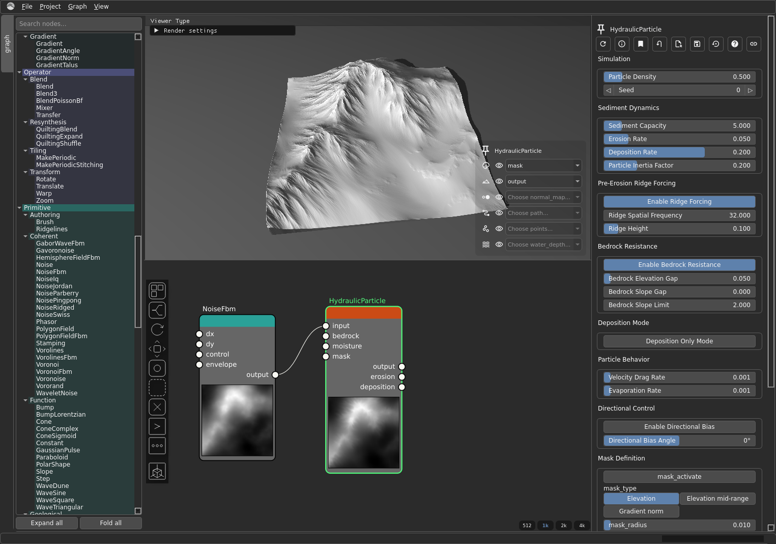
HydraulicParticle has several outputs (output, erosion, deposition); for this walkthrough you only need output — the eroded heightmap. That single output port is what feeds both branches of the fork.

Why: erosion is the step that turns generic noise into believable landforms.

Step 3 — Colour by elevation (ColorizeGradient)

Add a ColorizeGradient node (category Texture). Wire the eroded heightmap — HydraulicParticle's output — into the colouriser's level input, then pick a gradient (the colormap) to map elevation to colour.

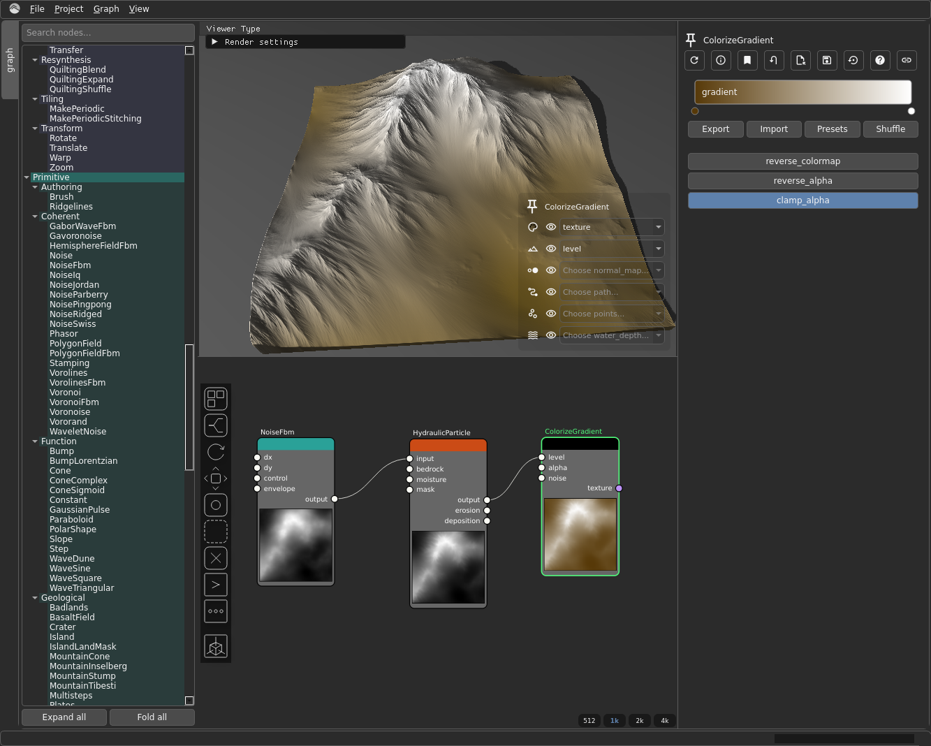
The data type changes here

Everything up to this point has been a heightmap (VirtualArray in the node reference). ColorizeGradient takes a heightmap in and emits a texture (VirtualTexture) out — an RGBA image. This is where you leave heightmap-land for colour-land, and it is why the texture export hangs off ColorizeGradient while the raw export does not: a texture cannot be fed into a node that expects a heightmap. See Heightmaps & virtual arrays.

Why: colour turns the grayscale elevation field into a map you can actually read.

Step 4 — Export both outputs

Now the graph forks. You want two files: the raw heightmap for your engine, and the coloured map for reference. They come from two different points in the graph.

• ExportHeightmap (category Export) ← wire HydraulicParticle's output into its input. This is the raw, engine-ready elevation. Because it needs a heightmap (VirtualArray), it must branch off the eroded heightmap before ColorizeGradient, not after it.
• ExportTexture (category Export) ← wire ColorizeGradient's texture output into its texture input. This is the coloured map.

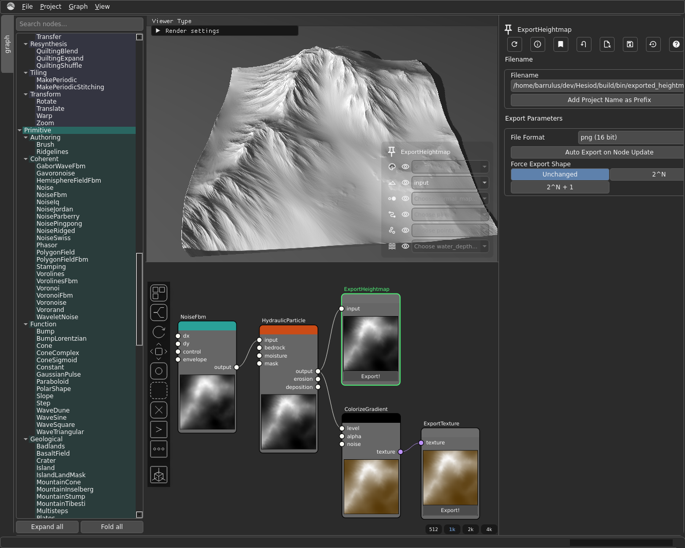
A single output port can drive multiple wires — that is how HydraulicParticle's output feeds both ExportHeightmap and ColorizeGradient at once. Drag a second wire out of the same port to make the second connection.

On each export node, set the file name in fname. ExportHeightmap also lets you choose a format; ExportTexture has a 16 bit toggle for higher colour depth. Both have an auto_export toggle — leave it on and the file is rewritten every time the graph updates.

Why: you usually want both — the raw heightmap to import into your engine, and the coloured version as a quick visual reference.

Next steps

• Core Concepts — the ideas behind what you just did (heightmaps, masks, tiling, broadcast).
• Node reference — every node, with its input/output ports and parameters.
• Building a "patch of graphs" — the advanced worldbuilding track: stitching several graphs into one large world.